|
<< Click to Display Table of Contents >> Traffic |
  
|
|
<< Click to Display Table of Contents >> Traffic |
  
|
Traffic is an important element of input. One should remember that the traffic of light vehicles, such as passenger cars, has a minimum influence on the pavement and as such it can be disregarded. For this reason cncPAVE concentrates on heavy vehicles (HV). There are seven major aspects related to heavy-vehicle traffic to be considered:
•Number of heavy vehicles expected to use the pavement initially, ADTT0, in HV/day;
•Growth of HV traffic over the period under study, g, in % p.a.;
•Average speed of heavy vehicles, V, in km/h;
•Average number of axles per heavy vehicle, aph;
•Wheel configuration (and the average lateral distance between wheels in case of dual wheels) c, in mm;
•Contact pressure applied to the pavement by heavy-vehicle wheels, p, in MPa; and
•Distribution of heavy-vehicle axle loads, in tons.
The seven aspects are discussed in some detail below.
1. Magnitude of the initial HV traffic, i.e the average daily HV traffic at the beginning of the first year of operation (after construction or rehabilitation), ADTT0, in HV/day, is input constant no. 2.
2. The average annual growth rate of HV traffic, g, in percent per annum, is input variable no. 12.
Two traffic-growth models are available in the cncPAVE program - (a) linear and (b) exponential. The user should click the appropriate radio button. The buttons are located at the top of the Axle Loads Page.
If the linear traffic growth is selected then the future average daily traffic is calculated as
![]()
If the exponential traffic growth is selected then the future average daily traffic is calculated as
![]()
where
ADTT0 average daily truck traffic at the beginning (time zero), HV/lane/day
ADTTn average daily truck traffic after n years, HV/lane/day
g growth factor, e.g. 1.045 for a 4.5 % p.a. rate of growth
n period of growth in years
(a) Linear traffic growth model
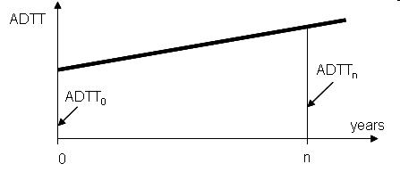
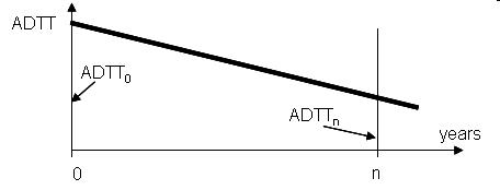
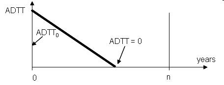
The calculations for the linear traffic-growth model are based on Eq.1a. Three cases are considered separately, viz.
(i) positive traffic growth, as shown below

(ii) negative traffic growth with ADTTn at the time n being still greater than zero, as shown below

(iii) negative traffic growth with ADTTn becoming zero before the time n, as shown below

In cases (i) and (ii) the total number of heavy vehicles that travel on the pavement during the period of n years is calculated from the area of the trapezium
ADTT0 - ADTTn - n - 0;
whereas in case (iii) from the area of the triangle
ADTT0 - 0 - 0.
(b) Exponential traffic-growth model
In case of the exponential traffic growth model the cncPAVE program assumes a steady continuous traffic growth expressed as a power function of time, Eq.1b. The traffic growth may be positive, zero, or negative.
The total number of heavy vehicles (HV) traveling on the pavement during a period n is obtained from Eq.1b, by integration and multiplication
TOTHVn = 365.25 . ADTT0 . (gn - 1) / ln (g) (2)
The total number of heavy vehicles present during the period t1 years from time zero to the first rehabilitation is
TOTHVt1 = 365.25 . ADTT0 . (gt1 - 1) / ln (g) (3)
If a rehabilitation action was carried out previously at a time previous, the next rehabilitation action will be required at a time next, after the number of heavy vehicles TOTHVt1 have again traveled on the road. The time next can be calculated from the following equation
TOTHVnext = TOTHVprevious + TOTHVt1 (4)
365.25 . ADTT0 .(g ynext -1) / ln (g) = 365.25 . ADTT0 . (gprevious - 1) / ln (g) + 365.25 . ADTT0 . (gt1 - 1) / ln (g) (5)
gnext - 1 = gprevious - 1 + gt1 -1 (6)
gnext = gprevious + gt1 -1 (7)
next . ln (g) = ln (gprevious + gt1 - 1) (8)
next = ln (gprevious + gt1 - 1) / ln (g) (9)
Note that g, previous and t1 in the above Eq.9 are all known, so that the time next can be determined. If traffic growth is zero then g = 1, and next = previous + t1.
Next times, both in case of the linear and exponential traffic growth, are calculated throughout the assumed life period of the pavement, and are used for the evaluation of the present worth of the rehabilitation action carried out at the respective next time. The results are shown in the table called ‘Typical rehabilitation schedule’ that is presented on the Facts Page.
In general, the exponential model yields HV traffic figures higher than those of the linear model. For a long period till the next intervention (such as 15 or 20 years), combined with high HV traffic growth rate (such as 8 % p.a. or more), the exponential model may produce an unrealistic magnitude of the future ADTT. For this reason the linear model is preferable unless there is a strong indication that in the given case the traffic is expected to grow steadily and continuously in a manner similar to that of money deposited in a bank at fixed interest .
3. Average speed of HV, V, in km/h, is input variable no. 13. A typical value is V = 80 km/h. Remember that low speeds are more detrimental to the pavement than high ones.
4. Average number of axles per HV, aph, is input constant no.3. High values of aph are more detrimental to the pavement than small ones.
When a traffic situation is selected on the Axle Loads Page, cncPAVE supplies the appropriate average number of axles automatically. This figure will appear on the Control Page, in the space for input constant no. 3, where it can be edited. The average axles/HV also appear among the characteristics printed below the graph on the Axle Loads Page. These values, together with other traffic characteristics, come from the 2005 data of the nation-wide WIM (weigh-in-motion) traffic monitoring program - see Ref.10.
5. Although small lateral wheel distances are more detrimental to the pavement than large ones, cncPAVE assumes dual-wheel configuration with the lateral distance c fixed at a typical value of 300 mm. For this reason c does not appear among variables or constants; it is not user-selectable.
6. Contact pressure applied to the pavement by heavy-vehicle wheels, p, in MPa, is variable no. 14. A typical value of contact pressure is 0.70 MPa. High pressures are more detrimental to the pavement than low ones.
7. Distribution of axle loads. The user may choose one of the several typical HV axle load distributions presented on the Axle Loads Page. Should none of the typical distributions be applicable to the studied case, cncPAVE will help the user to enter his or her own distribution of axle loads, as described in the above topic.